40 row labels in excel pivot table

excel - Custom row labels in PivotTable - Stack Overflow 1. you can give nicknames to the fields that you are checking which populate the pivot table. If you go the pivot table data and right click you can change the value field settings to give a custom name to a row/series but I do not know about individual data points. path: pivot table data => right click => select Field Settings => edit custom name. How to Move Excel Pivot Table Labels Quick Tricks - Contextures Excel … 12-07-2021 · Move Pivot Table Labels. This short video shows 3 ways to manually move the labels in a pivot table, and the written instructions are below the video. Drag a Label. Use Menu Commands. Type over a Label. Drag Labels to New Position. To move a pivot table label to a different position in the list, you can drag it: Click on the label that you want ...

Repeat item labels in a PivotTable - support.microsoft.com Right-click the row or column label you want to repeat, and click Field Settings. Click the Layout & Print tab, and check the Repeat item labels box. Make sure Show item labels in tabular form is selected. Notes: When you edit any of the repeated labels, the changes you make are applied to all other cells with the same label.

Row labels in excel pivot table

Quick tip: Rename headers in pivot table so they are presentable 15-03-2018 · Pivot tables are fun, easy and super useful. Except, they can be ugly when it comes to presentation. Here is a quick way to make a pivot look more like a report. Just type over the headers / total fields to make them user friendly. See this quick demo to understand what I mean: So simple and effective. Pivot Table "Row Labels" Header Frustration Pivot Table "Row Labels" Header Frustration. Hi Everyone please help I can't change my headers from Row Labels in a Pivot Table. Using Excel 365. Labels: How To Show Row Labels In Pivot Table Excel | Brokeasshome.com How To Control Excel Pivot Table With Field Setting Options Grouping Sorting And Filtering Pivot Data Microsoft Press Pivot Table Headings That Say Column Row Instead Of Actual Label You Use The Field List To Arrange Fields In A Pivottable

Row labels in excel pivot table. Multiple row labels on one row in Pivot table - MrExcel Message Board I figured it out - Right click on your pivot table and choose pivot table options/display. Click on "Classic PivotTable layout" Then click on where it is subtotaling your row label and uncheck the subtotal option. D dudeshane0 New Member Joined Oct 23, 2014 Messages 1 Jan 19, 2015 #6 Gerald Higgins said: How to Group Rows in Excel Pivot Table (3 Ways) - ExcelDemy Now, select any date in the PivotTable and then right-click. Then, select Group. After that, excel will automatically detect the starting and ending dates for grouping. You can change them as required. Then, select Days and Months to group By. Next, hit OK. Finally, the rows of dates in the PivotTable will be grouped as follows. Pivot Table Row Labels In the Same Line - Beat Excel! First make a pivot table with required fields. Arrange the fields as shown in left picture. Your initial table will look like right picture. Now click on "Error Code" and access field settings. First check "None" option in "Subtotals & Filters" tab to disable totals after every row. How to Move Pivot Table Labels - Contextures Excel Tips Jul 12, 2021 · Move Pivot Table Labels. This short video shows 3 ways to manually move the labels in a pivot table, and the written instructions are below the video. Drag a Label. Use Menu Commands. Type over a Label. Drag Labels to New Position. To move a pivot table label to a different position in the list, you can drag it: Click on the label that you want ...

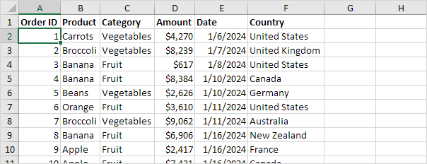
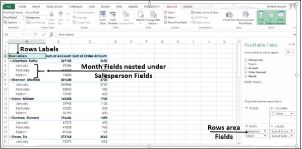
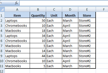
Excel Pivot Table Subtotals - Contextures Excel Tips 01-02-2022 · In the pivot table shown below, Service is in the Row Labels area, Lead Tech is in the Column Labels area, and Labor Cost is in the Values area. Because Service is the only field in the Row Labels area, it has no subtotal. Multiple Row Fields. When you add another field to the Row Labels area, a subtotal is automatically created for the first ... MS Excel 2016: How to Create a Pivot Table - TechOnTheNet Finally, we want the title in cell A1 to show as "Order ID" instead of "Row Labels". To do this, select cell A1 and type Order ID. Your pivot table should now display the total quantity for each Order ID as follows: Congratulations, you have finished creating your first pivot table in … How to Use Excel Pivot Table Label Filters - Contextures Excel Tips In an Excel pivot table, you might want to hide one or more of the items in a Row field or Column field. To do that, you could click the drop down arrow for the Row or Column Labels, to see the list of pivot items in that pivot field. Then, in the list, remove the check mark for items you want to remove. Pivot table row labels side by side - Excel Tutorials - OfficeTuts Excel You can copy the following table and paste it into your worksheet as Match Destination Formatting. Now, let's create a pivot table ( Insert >> Tables >> Pivot Table) and check all the values in Pivot Table Fields. Fields should look like this. Right-click inside a pivot table and choose PivotTable Options…. Check data as shown on the image below.

Quick tip: Rename headers in pivot table so they are ... Mar 15, 2018 · If you love working with pivot tables, check out below tips to become even more awesome. Sub-totals for only some levels; Change the order of pivot table row labels; First and last date of a sale with pivots; Introduction to pivot tables; Pivots from multiple tables; What is your favorite pivot tip? Please share in comments. Pivot table row labels in separate columns • AuditExcel.co.za So when you click in the Pivot Table and click on the DESIGN tab one of the options is the Report Layout. Click on this and change it to Tabular form. Your pivot table report will now look like the bottom picture and will be easier to use in other areas of the spreadsheet and in our opinion is also easier to read. Who wants to be a ... How to reverse a pivot table in Excel? - ExtendOffice To reverse the pivot table, you need to open PivotTable and PivotChart Wizard dialog first and create a new pivot table in Excel. 1. Press Alt + D + P shortcut keys to open PivotTable and PivotChart Wizard dialog, then, check Multiple consolidation ranges option under Where is the data that you want to analyze section and PivotTable option under What kind of report do you … Data Labels in Excel Pivot Chart (Detailed Analysis) 7 Suitable Examples with Data Labels in Excel Pivot Chart Considering All Factors 1. Adding Data Labels in Pivot Chart 2. Set Cell Values as Data Labels 3. Showing Percentages as Data Labels 4. Changing Appearance of Pivot Chart Labels 5. Changing Background of Data Labels 6. Dynamic Pivot Chart Data Labels with Slicers 7.

Excel Pivot Table Report - Sort Data in Row & Column Labels & in Values Area, use Custom Lists

Remove row labels from pivot table • AuditExcel.co.za Click on the Pivot table. Click on the Design tab. Click on the report layout button. Choose either the Outline Format or the Tabular format. If you like the Compact Form but want to remove 'row labels' from the Pivot Table you can also achieve it by. Clicking on the Pivot Table. Clicking on the Analyse tab.

Repeat Pivot Table Labels in Excel 2010 - Excel Pivot TablesExcel Pivot Tables

How to Insert a Blank Row in Excel Pivot Table | MyExcelOnline 17-01-2021 · Pivot Table reports are shown in a Compact Layout format as a default and if you have two or more Items in the Row Labels (e.g.Month & Customer), then the Pivot Table report can look very clunky…. There is a cool little trick that most Excel users do not know about that adds a blank row after each item, making the Pivot Table report look more appealing.

33 Pivot Table Blank Row Label - Labels Database 2020

How to filter date range in an Excel Pivot Table? - ExtendOffice Now you have filtered the date range in the pivot table. Notes: (1) If you need to filter out the specified date range in the pivot table, please click the arrow beside Row Labels, and then click Date Filters > Before/After/Between in the drop-down list as you need. In my case I select Date Filters > Between.

Group data in an Excel Pivot Table

Automatic Row And Column Pivot Table Labels - How To Excel At Excel The first thing to do is put your cursor somewhere in your data list Select the Insert Tab Hit Pivot Table icon Next select Pivot Table option Select a table or range option Select to put your Table on a New Worksheet or on the current one, for this tutorial select the first option Click Ok

Pivot Table Multiple Row Labels Side By Side

How to make row labels on same line in pivot table? - ExtendOffice Make row labels on same line with PivotTable Options You can also go to the PivotTable Options dialog box to set an option to finish this operation. 1. Click any one cell in the pivot table, and right click to choose PivotTable Options, see screenshot: 2.

Filtering Grand Total Amounts Within Excel Pivot Tables | AccountingWEB

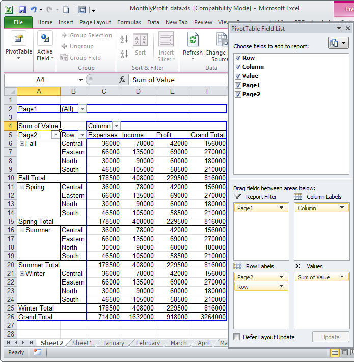
How to Create - wgqozc.meringhenuvole.it How to Create Pivot Tables and Pivot Charts in Excel 2019 A pivot table lets you see a snapshot of data and then see the same data in a different snapshot.Pivot tables allow you to answer several questions based on the same data. You set up a table to answer one question, and then you "pivot" the table to answer a second question. Set Up Data. Follow these steps, to change the layout: Select a ...

Design your Pivot Table in Excel | Excel in Excel

Changing Blank Row Labels - Excel Pivot Tables Select one of the Row or Column Labels that contains the text (blank). Type N/A in the cell, and then press the Enter key. Note: All other (Blank) items in that field will change to display the same text, N/A in this example. For more information on pivot tables, see the Pivot Table Topics on my Contextures web site.

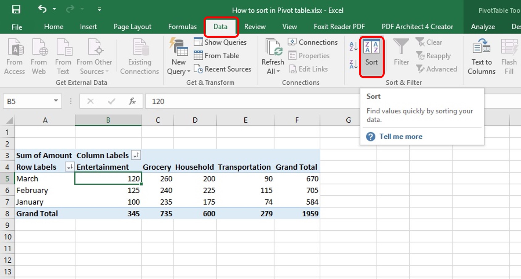
How to Sort Pivot Table | Custom Sort Pivot Table | A-Z, Z-A Order

Use column labels from an Excel table as the rows in a Pivot Table ... Highlight your current table, including the headers Then from the Data section of the ribbon, select From Table Highlight all the columns containing data, but not the Year column, and then select Unpivot Columns Close the dialog and keep the changes. Excel should place the unpivoted data into a new worksheet, looking something like this:

How to Use Excel Pivot Tables to Organize Data – excelhelpsblog

How to Flatten Data in Excel Pivot Table? - GeeksforGeeks Select a range that you want to flatten - typically, a column of labels. Highlight the empty cells only - hit F5 (GoTo) and select Special > Blanks. Type equals (=) and then the Up Arrow to enter a formula with a direct cell reference to the first data label. Instead of hitting enter, hold down Control and hit Enter.

Excel Pivot Tables (Example + Download) - VBA and VB.Net Tutorials, Education and Programming ...

How to rename group or row labels in Excel PivotTable? - ExtendOffice To rename Row Labels, you need to go to the Active Field textbox. 1. Click at the PivotTable, then click Analyze tab and go to the Active Field textbox. 2. Now in the Active Field textbox, the active field name is displayed, you can change it in the textbox. You can change other Row Labels name by clicking the relative fields in the PivotTable ...

Frequency Distribution in Excel - Easy Excel Tutorial

Move Row Labels in Pivot Table - Excel Pivot Tables Move Row Labels in Pivot Table When you add fields to the row labels area in a pivot table, the field's items are automatically sorted. See how you can manually move those labels, to put them in a different order. There's a video and written steps below. In the screen shot below, the districts are listed alphabetically, from Central to West.

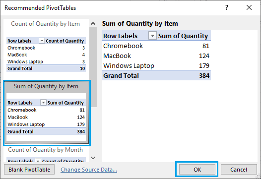
Advanced Excel - Pivot Table Recommendations - Tutorial Desk

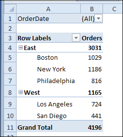
Pivot table - Wikipedia Row labels are used to apply a filter to one or more rows that have to be shown in the pivot table. For instance, if the "Salesperson" field is dragged on this area then the other output table constructed will have values from the column "Salesperson", i.e. , one will have a number of rows equal to the number of "Sales Person".

Choosing PivotTable Layouts | Microsoft Excel - Pivot Tables

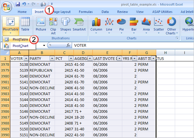
How to Create Excel Pivot Table (Includes practice file) Jun 28, 2022 · The area to the left results from your selections from [1] and [2]. You’ll see that the only difference I made in the last pivot table was to drag the AGE GROUP field underneath the PRECINCT field in the Row Labels quadrant. How to Create Excel Pivot Table. There are several ways to build a pivot table.

How to Create Pivot Table in Excel

get a row label from pivot table - Microsoft Tech Community Creating PivotTable add data to data model by checking Create PivotTable and after that convert it to cube formulas. Now you may take these formulas and convert it to form you need, for example in H3 it could be =CUBEVALUE( "ThisWorkbookDataModel", CUBEMEMBER("ThisWorkbookDataModel", " [Measures].

Repeat Pivot Table Labels in Excel 2010 – Excel Pivot Tables

Remove PivotTable Duplicate Row Labels [SOLVED] Re: Remove PivotTable Duplicate Row Labels. Sometimes when the cells are stored in different formats within the same column in the raw data, they get duplicated. Also, if there is space/s at the beginning or at the end of these fields, when you filter them out they look the same, however, when you plot a Pivot Table, they appear as separate ...

[5 Steps] How To Make Ranking Charts With Excel Pivot Tables - Moz

How to rename group or row labels in Excel PivotTable? - ExtendOffice To rename Row Labels, you need to go to the Active Field textbox. 1. Click at the PivotTable, then click Analyze tab and go to the Active Field textbox. 2. Now in the Active Field textbox, the active field name is displayed, you can change it in the textbox.

How Do Pivot Tables Work? - Excel Campus | Pivot table, Row labels, Excel

Pivot table - Wikipedia A pivot table usually consists of row, column and data (or fact) fields.In this case, the column is ship date, the row is region and the data we would like to see is (sum of) units.These fields allow several kinds of aggregations, including: sum, average, standard deviation, count, etc.In this case, the total number of units shipped is displayed here using a sum aggregation.

Share :