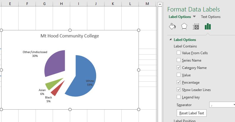
42 use the format data labels task pane to display category name and percentage data labels
How to show percentages on three different charts in Excel To convert the calculated decimal values to percentages, right-click on the selected cells and click Format Cells. Alternatively, press CTRL+1 on the keyboard to open the Format Cells dialogue box. 3. In the Format Cells dialogue box, make sure that the Number tab is selected and in the Category list select Percentage. Share Format Data Labels Display Outside End data - Chegg Close the Chart Elements menu. Use the Format Data Labels task pane to display Percentage data labels and remove the Value data labels. Close the task pane.
Send all sites not included in the Enterprise Mode Site List to ... Use DNS name resolution when a single-label domain name is used, by appending different registered DNS suffixes, if the AllowSingleLabelDnsDomain setting is not enabled. Use DNS name resolution with a single-label domain name instead of NetBIOS name resolution to locate the DC; Allow cryptography algorithms compatible with Windows NT 4.0
Use the format data labels task pane to display category name and percentage data labels
Excel Macros - Quick Guide - Tutorials Point Type the group name in the Display name dialog box and click OK. The new group name changes to Personal Macros (custom). Click Macros in the left pane under Choose commands from. Select your macro name, say – MyFirstMacro from the macros list. Click the Add button. The macro will be added under the Personal Macros (Custom) group. How to show data label in "percentage" instead of - Microsoft Community Select Format Data Labels Select Number in the left column Select Percentage in the popup options In the Format code field set the number of decimal places required and click Add. (Or if the table data in in percentage format then you can select Link to source.) Click OK Regards, OssieMac Report abuse 8 people found this reply helpful · Advanced Excel - Quick Guide - Tutorials Point Alternatively, you can also click on More Options available in the Data Labels options to display the Format Data Label Task Pane. The Format Data Label Task Pane appears. There are many options available for formatting of the Data Label in the Format Data Labels Task Pane. Make sure that only one Data Label is selected while formatting. Step 9 ...
Use the format data labels task pane to display category name and percentage data labels. Amazon EC2 FAQs - Amazon Web Services Use ec2-cancel-export-task to cancel an export task prior to completion. Q. Are there any other requirements when exporting an EC2 instance using VM Import/Export? You can export running or stopped EC2 instances that you previously imported using VM Import/Export. If the instance is running, it will be momentarily stopped to snapshot the boot ... Display the percentage data labels on the active chart. - YouTube Display the percentage data labels on the active chart.Want more? Then download our TEST4U demo from TEST4U provides an innovat... Excel 3-D Pie charts - Microsoft Excel 2016 - OfficeToolTips If you want to create a pie chart that shows your company (in this example - Company A) in the greatest positive light: Do the following: 1. Select the data range (in this example, B5:C10 ). 2. On the Insert tab, in the Charts group, choose the Pie button: Choose 3-D Pie. 3. Right-click in the chart area, then select Add Data Labels and click ... Success Essays - Assisting students with assignments online Get 24⁄7 customer support help when you place a homework help service order with us. We will guide you on how to place your essay help, proofreading and editing your draft – fixing the grammar, spelling, or formatting of your paper easily and cheaply.
Build media apps for cars | Android Developers Jan 07, 2022 · Supply short but meaningful labels for each tab item. Keeping labels short reduces the chance of the strings getting truncated. Display media artwork. Artwork for media items must be passed as a local URI using either ContentResolver.SCHEME_CONTENT or ContentResolver.SCHEME_ANDROID_RESOURCE. This local URI must resolve to either a … Format Data Labels in Excel- Instructions - TeachUcomp, Inc. To format data labels in Excel, choose the set of data labels to format. To do this, click the "Format" tab within the "Chart Tools" contextual tab in the Ribbon. Then select the data labels to format from the "Chart Elements" drop-down in the "Current Selection" button group. Excel tutorial: How to use data labels When first enabled, data labels will show only values, but the Label Options area in the format task pane offers many other settings. You can set data labels to show the category name, the series name, and even values from cells. In this case for example, I can display comments from column E using the "value from cells" option. How to Create Progress Charts (Bar and Circle) in Excel Step #4: Insert custom data labels. Now, replace the default data labels with the respective percentages for each progress bar. To do that, right-click on any of the data labels and choose "Format Data Labels." In the task pane that appears, do the following: Navigate to the Label Options tab. Check the "Value From Cells" box. In the ...
How do you format data series in Excel? - FAQ-ALL Select the decimal number cells, and then click Home > % to change the decimal numbers to percentage format . 7. Then go to the stacked column, and select the label you want to show as percentage , then type = in the formula bar and select percentage cell, and press Enter key. How to format data series independently in Excel 4.2 Formatting Charts - Beginning Excel, First Edition On the Design tab select the Add Chart Element button, then Data Labels, then Outside End (see Figure 4.36.) Click on one of the Data Labels. Note that all of the data labels for that data series are selected. Using the Home ribbon, change the font to Arial, Bold, size 9. Click on one of the data labels for the other data series. Changing the order of items in a chart - PowerPoint Tips Blog 2. Individually change the order of items. You can manage the order of items one by one if you don't want to reverse the entire set. Follow these steps: With the chart selected, click the Chart Tools Design tab. Choose Select Data in the Data section. The Select Data Source dialog box opens. You can only change the values on the left side of ... Solved step by step instruction 2 A pie chart is an | Chegg.com Use the Insert tab to create a pie chart from the Question: step by step instruction 2 A pie chart is an effective way to visually illustrate the percentage of the class that earned A, B, C, D, and F grades. Use the Insert tab to create a pie chart from the This problem has been solved! See the answer step by step instruction Expert Answer
4.1 Choosing a Chart Type – Beginning Excel, First Edition
Excel - Quick Guide - Tutorials Point Column labels − A field that has a column orientation in the pivot table. Each item in the field occupies a column. Report Filter − You can set the filter for the report as year, then data gets filtered as per the year. Row labels − A field that has a row orientation in the pivot table. Each item in the field occupies a row.
Post a Comment for "42 use the format data labels task pane to display category name and percentage data labels"